5. The cases of southward transport and deposition of semivolatile organics (SVO’s) from multiple sources in April.
The prevailing weather conditions in April 1999 were changeable with
frequent rainfall mainly over the central and to a lesser extent over the
southern Balkan area. This may have increased wet deposition in the proximity
of the emission sources. During this month, low pressure systems dominated the
area, interrupted by a few transitory ridges of high pressure. As a result,
periods of north-westerly flow, favouring
transport of air masses from former Yugoslavia to the south, were
limited. On the 7th of April, a ridge of high pressure resulted to
drier weather in the Balkans with winds blowing from northerly directions.
These conditions lasted for not more than 1.5 days. Short-lived spell with
northerly flow also occurred on 18-19 April 1999.
The combination of the information about the bombing with estimations about emissions from explosions found in the literature (Church, 1969) resulted to the following emission scenarios:
·
April 4-7:
Multiple
sources scenario.
(a)
April 4: One
line source from 100 m to 500 m above ground level (AGL) over Belgrade (fuel storage), one over Novi Sad (oil refinery), one over
Bogutovac (fuel storage) and one over Smederevo (petrochemical industry
installations). The emission started at April 4,
2.00 UTC and lasted 12 hours.
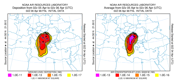
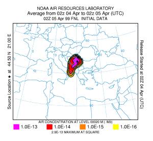
Figure 8.1a:
Time integrated concentrations calculated with HYSPLIT_4 modeling system for April 4. The stars indicate the
geographic position of the sources. A line source is assumed at each location
which stretches from 100 to 500 m AGL. The concentrations are given in
relative units, corresponding to an emission rate of 1 unit of pollutant per
hour.
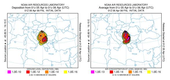
(b) April 5: One
line source from 100 m to 500 m above ground level (AGL) over Sombor (fuel storage), one over Novi Sad (power station)
and one over Nis (warehouse). The
emission started at April 5, 1.00
UTC and lasted 12 hours.
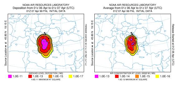
Figure 8.1b:
Time integrated concentrations calculated with HYSPLIT_4 modeling system for April 5. The stars indicate the
geographic position of the sources. A line source is assumed at each location
which stretches from 100 to 500 m AGL. The concentrations are given in
relative units, corresponding to an emission rate of 1 unit of pollutant per
hour.
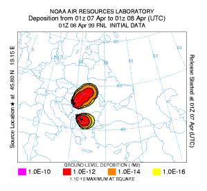
(c)April 6: One
line source from 100 m to 500 m above ground level (AGL) over Sombor
(petrochemical industry warehouse), one over Novi Sad (bitumen storage &
power station) and one over
Prizren (cement plant). The emission started at April 6,
1.00 UTC and lasted 12 hours.
Figure
8.1c: Time integrated concentrations
calculated with HYSPLIT_4 modeling system for April 18-20. The stars indicate the
geographic position of the sources. A line source is assumed at each location
which stretches from 100 to 500 m AGL. The concentrations are given in
relative units, corresponding to an emission rate of 1 unit of pollutant per
hour.
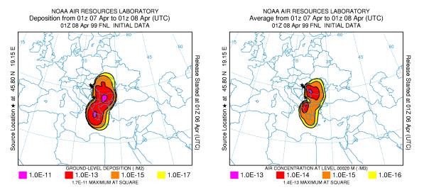
(d) April 7: One line source from 100 m to 500 m above ground level (AGL) over Pristina
(fuel storage), one over Novi Sad (industrial company) and one over Sombor (fuel storage). The
emission started at April 7, 1.00 UTC and lasted 12 hours.
 |
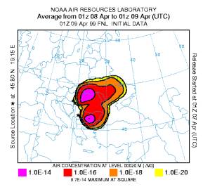 |
Figure 8.1d: Time integrated concentrations calculated with HYSPLIT_4 modeling system for April 18-20. The stars indicate the geographic position of the sources. A line source is assumed at each location which stretches from 100 to 500 m AGL. The concentrations are given in relative units, corresponding to an emission rate of 1 unit of pollutant per hour.
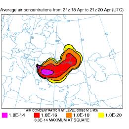
· April 18–20: One line source from 100 m to 500 m AGL over Pristina and one over Kursumlija. The emission started at April 18, 21 UTC and lasted 12 hours.
 |
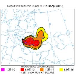 |
Figure 8.2: Time integrated concentrations calculated with
HYSPLIT_4 modeling system for April 18-20. The stars indicate the geographic
position of the sources. A line source is assumed at each location which
stretches from 100 to 500 m AGL. The concentrations are given in relative
units, corresponding to an emission rate of 1 unit of pollutant per hour.
As mentioned before, aerosol
samples were collected at Xanthi, Greece (41.15 oN, 25 oE),
on a moving glass fiber filter band
GF10 6 cm width with 1 μm nominal
porocity of a high volume sampler (Rapsomanikis et al, 1999). They were also
collected by a PM2.5 μm High
Volume Dichotomous Virtual Impactor (HVDVI) (Solomon et al., 1983) on glass fiber 90 mm diameter GF/F filters with
nominal porocity of 1 μm. Parts
of the filter band and parts of the HVDVI filters, constituting of 24h samples,
were analysed using high resolution gas chromatography coupled with high
resolution mass spectrometry by Scientific Analysis Laboratories Ltd (SAL),
U.K. The background concentrations for the compounds of interest in the area
was estimated from samples of filter band for days that air masses originated
from the former Yugoslavia, before the onset of the conflict.
The following SVO’s were
quantitatively determined:
Dioxins and furans: 2,3,7,8-TCDD; 1,2,3,7,8-PeCDD; 1,2,3,6,7,8-HxCDD;
1,2,3,4,7,8-HxCDD; 1,2,3,7,8,9-HxCDD; 1,2,3,4,6,7,8-HpCDD; OCDD; 2,3,7,8-TCDF;
1,2,3,7,8-PeCDF; 2,3,4,7,8-PeCDF; 1,2,3,4,7,8-HxCDF; 1,2,3,6,7,8-HxCDF;
2,3,4,6,7,8-HxCDF; 1,2,3,7,8,9-HxCDF; 1,2,3,4,6,7,8-HpCDF; 1,2,3,4,7,8,9-HpCDF;
OCDF.
PCB’s: Tri-, tetra-, penta-, hexa- and
hepta-chlorobiphenyls
PAH’s: Napthalene, Acetapthylene, Acenaphthene, Fluorene, Phenanthene,
Anthralene, Fluoranthene, Pyrene, Benzo(a)anthracene, Chrysene, Benzo(b/k)fluoranthene,
Benzo(a)pyrene, Indeno(123-cd)pyrene, Benzo(ghi)perylene,
Dibenzo(ah)anthracene.
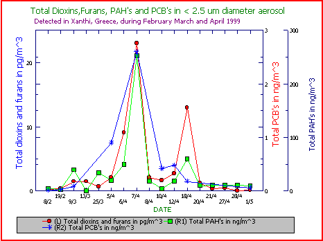
Figure 9a: Time series of 24hr
integrated aerosol samples for total dioxins, furans, PCB's and PAH's. For the
dates that data are not depicted, concentrations were not detectable.
Figure 9a, adapted from
Rapsomanikis et al. (1999), shows
atmospheric concentrations of total dioxins, furans, PCB’s and PAH’s. As can be
seen from the time series of SVO’s in figure 9a, the two events can be clearly distinguished from background
values. In the first episode concentrations of total dioxins, furans and PCB’s
increased ten fold, whilst concentrations of total PAH’s increased twenty
fold. The second episode is less
prominent and increases were three fold for dioxins, furans and PAH’s whilst no
increase was observed for PCB’s. The onset and end of these events is
consistent with dispersion calculations depicted in figures 8.1a-d and 8.2.
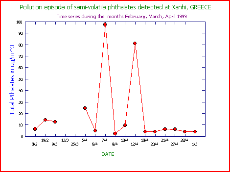
Figure 9b: Time series of 24hr
integrated aerosol samples for total phthalates. For the dates that data are
not depicted, concentrations were not detectable.
Phthalates are
used as plasticizers in a variety of plastics and are emitted in the atmosphere
after burning of plastics in fires and / or municipal incinerators. Their toxicity
and atmospheric concentrations are well documented with total concentrations
ranging from 0.3 – 1.0 μg/m3
(California EPA, 1994,Dugenest et al.,
1999, Fredricson et al., 1999). Total
values for the concentration of the following phthalates were determined in the
atmosphere of Xanthi: Dimethyl phthalate, Di-n-butyl phthalate, Butyl benzyl
phthalate, Bis (2 ethyl hexyl)
phthalate Diethyl phthalate. Their time series in April is shown in
figure 9b.
It should be
emphasized that these events could not have been caused by pollution from
nearby sources because of the unique combination of detected pollutant species
as seen in figure 9a. Lack of similar measurements in the Balkans prevented any
attempt to carry out a risk assessment analysis and a further validation of the
model results.
|
|
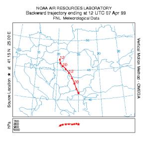
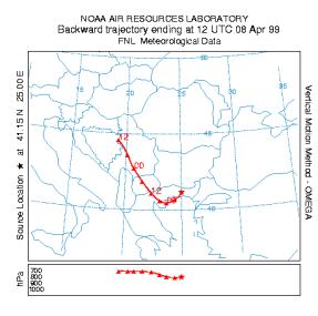
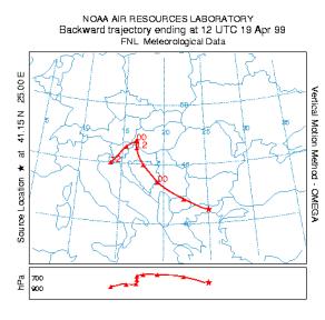
| Figure 10. Back trajectories at 850 hPa with end point in Xanthi, Greece, calculated with HYSPLIT_4 modeling system for April 7 and 8, respectively. The star indicates the geographic position of the source and the triangles the position of the air pollutants in 12hrs time intervals. | |
|
|
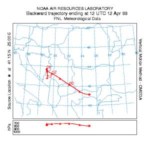
| Figure 11. Back trajectories at 850 hPa with end point in Xanthi, Greece, calculated with HYSPLIT_4 modeling system for April 12 and 19, respectively. The star indicates the geographic position of the source and the triangles the position of the air pollutants in 12hrs time intervals. | |
| In concluding this paragraph, we have calculated back-trajectories with starting level at 850 hPa (~1500 m height) calculated for the days of interest, with the Langrangian model HYSPLIT_4 (Draxler, 1997, Draxler, 1998). Such conditions were met for example with end point in Xanthi at 850 hPa (1500m height above sea level) on April 7, 8, 12, and 19 as seen in figures 10-11. These figures clearly show the origin of the air masses which moved southward carrying toxic gases which were measured at Xanthi.. | |